Clustering In Machine Learning
Machine learning has two major types: supervised and unsupervised learning. Clustering falls under unsupervised learning, where the goal is to group similar data points together. Unlike supervised learning, where labeled data is used to train models, clustering does not have predefined labels. It helps in pattern discovery, data segmentation, and anomaly detection.
Clustering is widely used in different industries, including customer segmentation in marketing, anomaly detection in cybersecurity, and document classification in natural language processing.
What is Clustering in Machine Learning?
Clustering is an unsupervised machine learning technique used to group similar data points into clusters. A cluster is a group of objects that share similar characteristics. The primary goal of clustering is to identify hidden structures in data.
Key Concepts of Clustering
- Unsupervised Learning: Clustering does not require labeled data, making it useful for discovering patterns and trends in large datasets.
- Grouping Similar Data Points: The algorithm identifies similarities between data points and groups them into clusters.
- Distance Metrics: Clustering relies on mathematical distance measures such as Euclidean distance, Manhattan distance, and cosine similarity to determine the closeness of data points.
- Cluster Centroids: Many clustering algorithms, such as K-Means, compute centroids that represent the center of a cluster.
- High-Dimensional Data Handling: Clustering algorithms can be applied to multi-dimensional data spaces, making them useful in various domains such as image segmentation and customer segmentation.
Why is Clustering Important?
- Data Segmentation: Helps in dividing a large dataset into meaningful subgroups.
- Anomaly Detection: Identifies outliers in data, useful for fraud detection and cybersecurity.
- Pattern Recognition: Finds hidden patterns in data for better decision-making.
- Feature Engineering: Used to create new features that enhance machine learning models.
Example of Clustering
The following image represents an example of clustering in machine learning. It visually demonstrates how data points are grouped into different clusters based on their similarities.
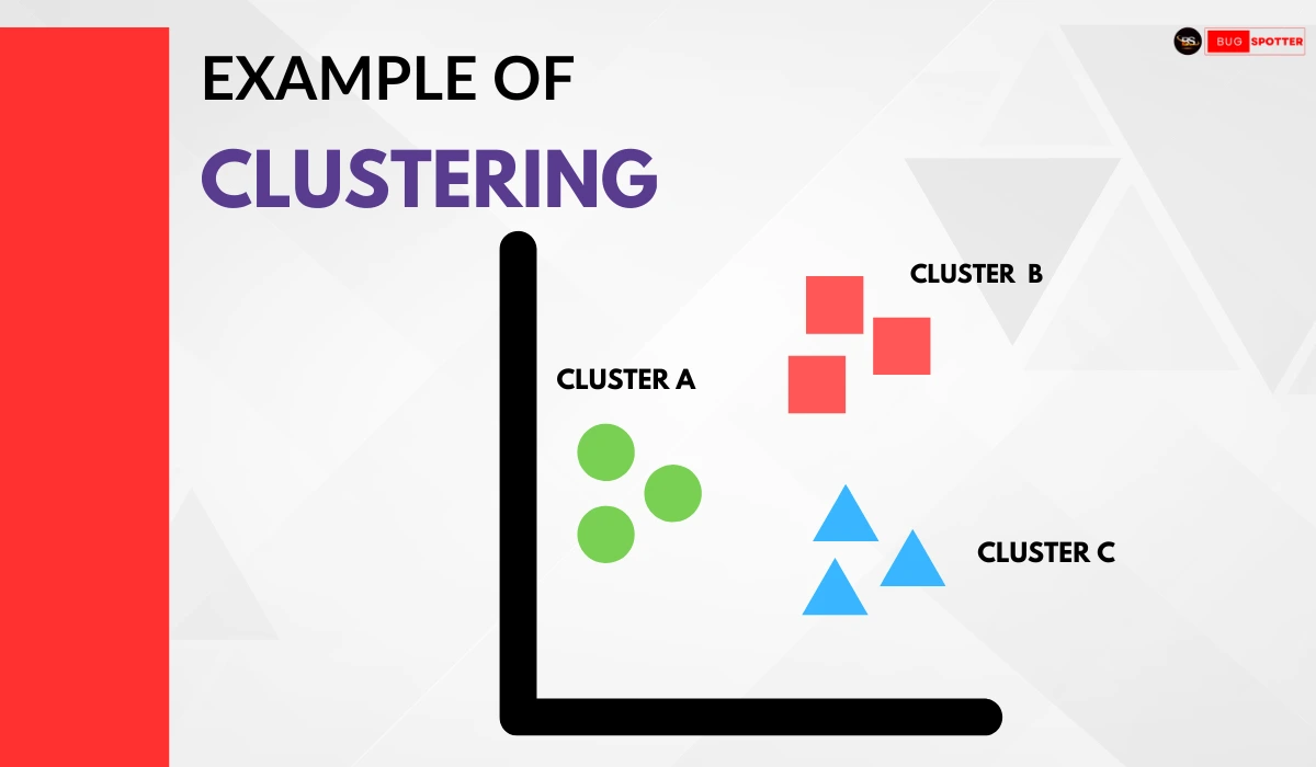
Explanation of the Clustering Example:
- The image consists of three distinct clusters: Cluster A, Cluster B, and Cluster C.
- Cluster A (Green Circles) represents a group of similar data points that are closely related.
- Cluster B (Red Squares) contains another set of similar points grouped together.
- Cluster C (Blue Triangles) is another distinct cluster with a separate group of points.
- Each shape represents a unique type of data, and clustering helps in identifying and grouping similar entities together.
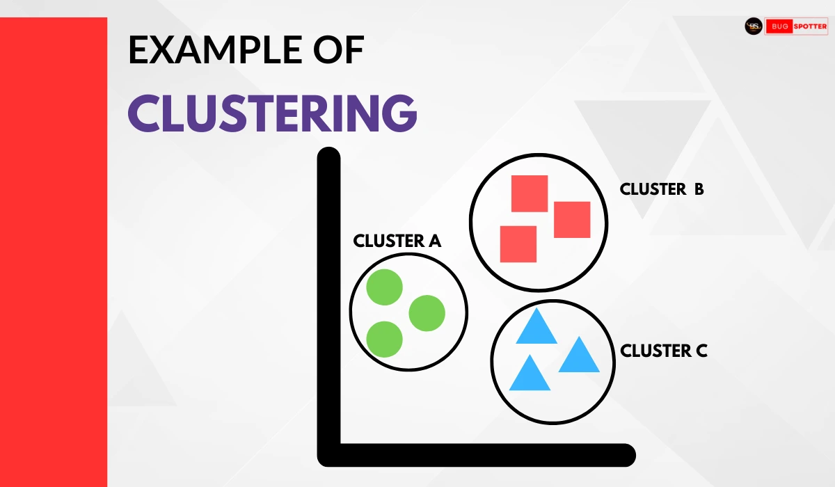
This example illustrates how clustering can be applied to categorize data points based on shared features, which is commonly used in applications like customer segmentation, pattern recognition, and data classification.
Real-World Analogy
Imagine you have a dataset of customers based on their shopping habits:
- Cluster A (Green Circles): Customers who frequently buy organic and health-conscious products.
- Cluster B (Red Squares): Customers who purchase high-end luxury items.
- Cluster C (Blue Triangles): Customers who buy electronic gadgets frequently.
By applying clustering algorithms like K-Means or DBSCAN, businesses can target each group differently, improving personalized marketing strategies.
Types of Clustering in Machine Learning
1. Hard Clustering
Hard clustering refers to a method where each data point is assigned to one and only one cluster. There is no overlap between the clusters in this approach. It’s a more strict way of clustering because each data point has a definite group assignment.
Key Characteristics:
- Exclusive Grouping: Every data point belongs to exactly one cluster.
- No Overlap: Once a data point is assigned to a cluster, it cannot belong to any other cluster.
Example:
Consider a business segmenting customers based on purchasing behavior. In hard clustering, each customer would be placed in a single group—say, “High Spend,” “Medium Spend,” or “Low Spend.” A customer would be placed in only one of these categories based on their spending habits. There’s no ambiguity; the customer is either in one cluster or another, but not both.
2. Soft Clustering (Fuzzy Clustering)
Soft clustering, also known as fuzzy clustering, allows data points to belong to multiple clusters, but with a degree of membership represented by a probability score. Rather than forcing a point into one cluster, soft clustering assigns a probability (or a fuzzy value) that shows how strongly a point belongs to each cluster.
Key Characteristics:
- Multiple Memberships: A data point can belong to multiple clusters simultaneously, with varying degrees of belonging.
- Probability Scores: Each data point has a degree of membership for each cluster, often expressed as a percentage or a number between 0 and 1.
Example:
In document classification, an article about AI in healthcare may belong to both a “Technology” cluster and a “Healthcare” cluster. The article could have a 60% probability of belonging to “Technology” and a 40% probability of belonging to “Healthcare.” This allows for flexibility in cases where categories overlap, and helps in understanding data with complex relationships.
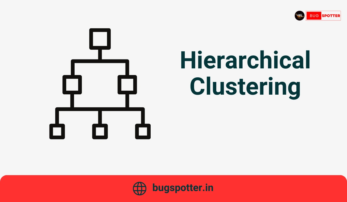
3. Hierarchical Clustering
Hierarchical clustering builds a tree-like structure of clusters, known as a dendrogram. This hierarchical approach doesn’t require a predefined number of clusters; it dynamically creates them through a process of merging or dividing clusters based on their similarities.
There are two main types of hierarchical clustering:
- Agglomerative Clustering: This is the most common form. It starts by treating each data point as its own individual cluster. Then, it iteratively merges the closest clusters based on their similarity. This continues until all points are grouped into a single cluster.
Example: Think of it like a family tree. Individual points (people) start as small clusters (nodes) and then progressively merge to form larger groups as you move up the tree.
- Divisive Clustering: This approach works the opposite way. It begins with all data points in one large cluster and recursively splits it into smaller clusters based on dissimilarity. It keeps dividing the data until the desired number of clusters is reached.
Example:
Imagine starting with a broad category (like “all animals”) and then progressively dividing it into more specific categories (e.g., mammals, reptiles, birds, etc.).
Use Case:
Hierarchical clustering is particularly useful in areas like bioinformatics (e.g., grouping genes with similar expression patterns), where the relationships between groups can be complex and require a detailed view.
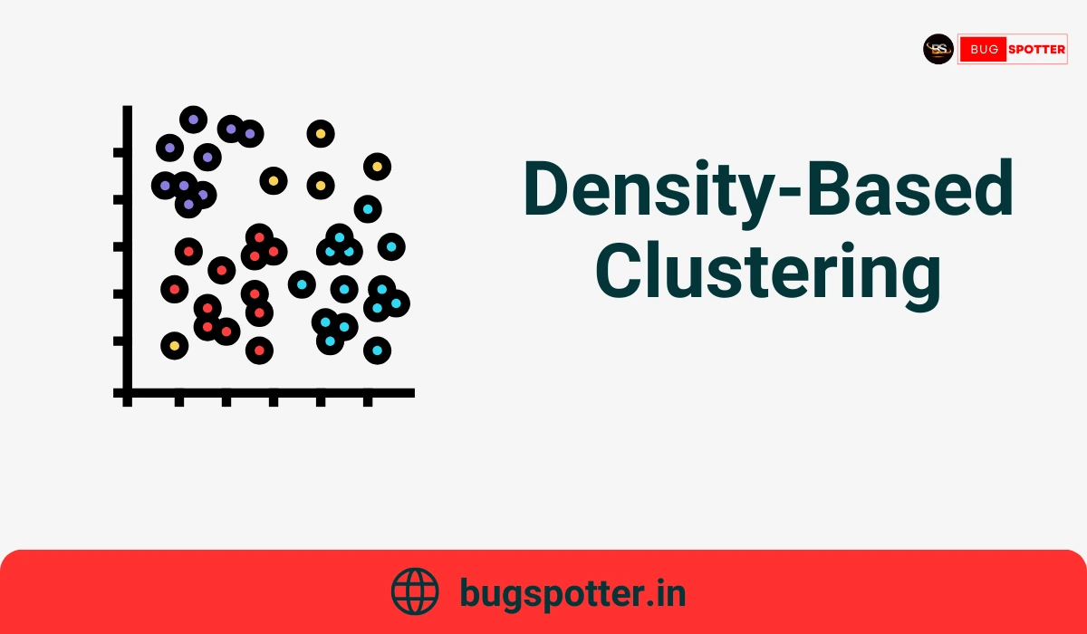
4. Density-Based Clustering
Density-based clustering forms clusters based on areas of high data point density, rather than on predefined shapes or distances. In this method, clusters are formed when data points are closely packed together, while outliers or points in low-density regions are treated as noise.
Key Characteristics:
- Clusters Formed by Density: Clusters are formed where data points are densely packed. These clusters may have irregular shapes, unlike the circular or spherical clusters that other methods might produce.
- Noise Identification: Data points in areas with low density are considered noise or outliers and are not assigned to any cluster.
Example:
DBSCAN (Density-Based Spatial Clustering of Applications with Noise) is one of the most popular density-based algorithms. It can find clusters with complex shapes, such as clusters in geographic data that may not form perfect circles. For example, DBSCAN could identify dense regions of earthquakes, with isolated points representing data that doesn’t fit into the main pattern (e.g., earthquake data from a different region).
Use Case:
DBSCAN is commonly used for anomaly detection, geographic data analysis, and situations where clusters are of varying shapes, such as detecting unusual patterns in network traffic (for cybersecurity).
5. Partition-Based Clustering
Partition-based clustering divides the dataset into a specific number of distinct clusters. This method assigns each data point to exactly one cluster, similar to hard clustering, but it differs in that it focuses on optimizing a certain criterion (like minimizing variance or maximizing similarity).
Key Characteristics:
- Fixed Number of Clusters (K): A predefined number of clusters (K) must be chosen before applying the algorithm.
- Cluster Assignment: Each data point is assigned to one of the K clusters based on a similarity metric, such as Euclidean distance.
Example:
K-Means clustering is a well-known partition-based algorithm. Suppose we want to group customers into K groups based on their spending behavior. If we set K=3, K-Means will group customers into three clusters: “High Spend,” “Medium Spend,” and “Low Spend.” The algorithm tries to minimize the variance within each cluster and maximize the variance between the clusters.
Use Case:
K-Means is widely used in applications like customer segmentation (as mentioned in your example), image compression (reducing the number of colors in an image), and market basket analysis (grouping products that are frequently bought together).
Types of Clustering Algorithms
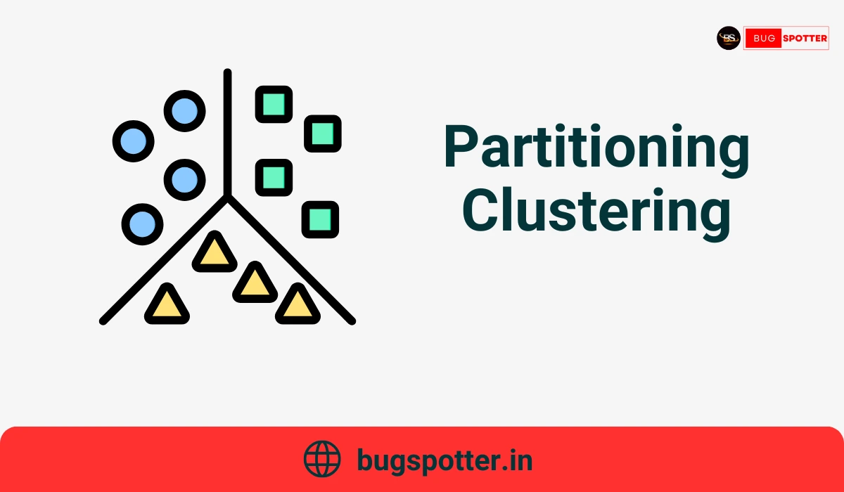
1. Partitioning Clustering
Partitioning clustering algorithms aim to divide a dataset into a predefined number of K disjoint clusters. These algorithms assign each data point to exactly one cluster, and the goal is to optimize a criterion to minimize the differences within each cluster and maximize the differences between clusters.
Key Characteristics:
- Predefined Number of Clusters (K): The user must specify the number of clusters before applying the algorithm.
- Exclusive Membership: Each data point is assigned to only one cluster.
- Optimization Objective: The algorithm works by minimizing the distance between data points and their cluster centroids.
How It Works:
K-Means is the most common partitioning algorithm. It starts by randomly initializing K centroids and then assigns each data point to the closest centroid. The centroids are updated by calculating the mean of the points assigned to each centroid, and the process continues until convergence.
K-Medoids is another popular partitioning algorithm, where medoids (representative points from the dataset) are chosen instead of centroids.r.
2. Density-Based Clustering
Density-based clustering algorithms focus on the density of data points in the data space to form clusters. Instead of requiring a predefined number of clusters, these algorithms create clusters by grouping points that are close to one another, with areas of low density considered as noise or outliers.
Key Characteristics:
- Density-Dependent: Clusters are formed based on the density of data points in a region. High-density areas form clusters, while low-density areas are treated as noise.
- No Need to Specify K: Unlike partitioning algorithms, density-based clustering does not require you to specify the number of clusters beforehand.
- Can Handle Arbitrary Shapes: Clusters can have arbitrary shapes and do not need to be circular or spherical.
How It Works:
DBSCAN (Density-Based Spatial Clustering of Applications with Noise) is one of the most popular density-based clustering algorithms. It works by identifying core points that have a minimum number of neighboring points within a specified radius (ε). Points within this neighborhood are grouped together into a cluster, and outliers (noise) are points that do not meet this density criterion.
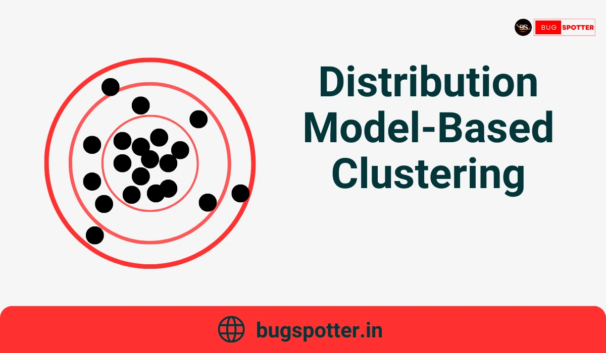
3. Distribution Model-Based Clustering
Distribution model-based clustering assumes that the data is generated by a mixture of different probability distributions. Each cluster is modeled as a distribution, typically a Gaussian distribution (or normal distribution), and the algorithm tries to estimate the parameters of these distributions.
Key Characteristics:
- Probabilistic Approach: Data points are assigned to clusters based on the probability that they belong to each distribution.
- Overlapping Clusters: Unlike other clustering algorithms, this method allows for overlapping clusters. A data point can have a certain probability of belonging to multiple clusters.
- Use of Statistical Models: The algorithm tries to fit a model (e.g., Gaussian Mixture Model or GMM) to the data by estimating the parameters of the distribution (mean, variance).
How It Works:
Gaussian Mixture Models (GMM) are the most common distribution model-based clustering algorithms. GMM assumes that data points come from a mixture of multiple Gaussian distributions. The algorithm uses the Expectation-Maximization (EM) algorithm to iteratively estimate the parameters of these distributions and assign probabilities to each data point belonging to a specific cluster.
4. Hierarchical Clustering
Hierarchical clustering builds a hierarchy of clusters, where clusters are nested within one another. The hierarchy is represented as a tree-like structure called a dendrogram, which allows you to visualize the clustering process at different levels of granularity.
Key Characteristics:
- No Need to Specify K: You do not need to specify the number of clusters in advance, making it flexible.
- Produces a Dendrogram: A tree-like structure that shows the relationships between clusters, with the ability to “cut” the tree at a specific level to define clusters.
- Can Be Agglomerative or Divisive: It can either start with individual data points and merge them into clusters (agglomerative) or start with one large cluster and split it into smaller ones (divisive).
How It Works:
Agglomerative Clustering (bottom-up) starts with each data point as its own cluster and iteratively merges the closest clusters based on a distance metric until all data points are in a single cluster.
Divisive Clustering (top-down) begins with all points in a single cluster and recursively splits the clusters into smaller ones.
Latest Posts
- All Posts
- Software Testing
- Uncategorized


Categories
- Artificial Intelligence (5)
- Best IT Training Institute Pune (9)
- Cloud (2)
- Data Analyst (55)
- Data Analyst Pro (15)
- data engineer (18)
- Data Science (104)
- Data Science Pro (20)
- Data Science Questions (6)
- Digital Marketing (4)
- Full Stack Development (7)
- Hiring News (41)
- HR (3)
- Jobs (3)
- News (1)
- Placements (2)
- SAM (4)
- Software Testing (70)
- Software Testing Pro (8)
- Uncategorized (33)
- Update (33)
Tags
- Artificial Intelligence (5)
- Best IT Training Institute Pune (9)
- Cloud (2)
- Data Analyst (55)
- Data Analyst Pro (15)
- data engineer (18)
- Data Science (104)
- Data Science Pro (20)
- Data Science Questions (6)
- Digital Marketing (4)
- Full Stack Development (7)
- Hiring News (41)
- HR (3)
- Jobs (3)
- News (1)
- Placements (2)
- SAM (4)
- Software Testing (70)
- Software Testing Pro (8)
- Uncategorized (33)
- Update (33)