Support Vector Machine in Machine Learning (SVM)

Machine learning has transformed the way we solve complex problems, especially in classification and regression tasks. One of the most powerful supervised learning algorithms used for classification is the Support Vector Machine (SVM).

SVM is widely used in applications such as image recognition, spam detection, sentiment analysis, and medical diagnosis due to its high accuracy and ability to handle both linear and non-linear data.

What is a Support Vector Machine (SVM)?

A Support Vector Machine (SVM) is a supervised machine learning algorithm that is used primarily for classification and regression tasks. It works by finding the optimal hyperplane that best separates the data points into different classes.

The key idea behind SVM is to find the decision boundary that maximizes the margin between different classes, ensuring that the classification is as robust as possible.

Imagine you want to divide two groups of objects (e.g., apples and oranges) based on their characteristics (e.g., size and weight). SVM helps find the best dividing line (called a hyperplane) to separate these groups.

In simple terms, SVM works by:

Finding the best boundary (hyperplane) that separates different classes.
Maximizing the distance (margin) between this boundary and the nearest data points.
Handling complex data by transforming it into a higher dimension if needed.

Key Terms in SVM

Hyperplane
Support Vectors
Margin

1. What is a Hyperplane?

A hyperplane is the decision boundary that separates different classes in an SVM model. It is a mathematical concept that extends beyond the traditional understanding of lines and planes.

Hyperplane in Different Dimensions
In 2D space (two features) → A hyperplane is a straight line that separates two classes.
In 3D space (three features) → A hyperplane is a flat plane that separates the points.
In higher dimensions (more than three features) → The hyperplane is an N-dimensional space that divides data.
Real-Life Example of a Hyperplane
Imagine you are organizing books in a library. You have two types of books: fiction and non-fiction. You arrange them on a shelf and draw an imaginary line between them to separate fiction from non-fiction.This imaginary line is equivalent to the hyperplane in an SVM classifier!
Mathematical Representation of a Hyperplane
A hyperplane in an N-dimensional space is represented as: w.x+b=0

Where:

w is the weight vector (defines the direction of the hyperplane).
x is the feature vector (data points).
b is the bias term (shifts the hyperplane).

The goal of SVM is to find the optimal hyperplane that best separates the classes while maximizing the margin.

2. What are Support Vectors?

Support Vectors are the most important data points in SVM. They are the data points that are closest to the hyperplane and define its position.

Since SVM aims to maximize the margin, only a few data points (support vectors) determine the placement of the hyperplane. Any other data points that are farther away do not influence the decision boundary.

Why Are Support Vectors Important?

They define the margin of the hyperplane.
They help in classification by ensuring robustness.
If we remove or change a support vector, the hyperplane may shift significantly.

Real-Life Example of Support Vectors

Imagine a tightrope walker balancing on a rope. The two poles holding the rope are like support vectors—they determine how tight or loose the rope (decision boundary) is.

Similarly, in SVM, support vectors determine the optimal position of the hyperplane.

3. What is Margin in SVM?

The margin is the distance between the hyperplane and the nearest support vectors.

A larger margin → Better generalization and robustness.
A smaller margin → Higher risk of overfitting.

Types of Margins in SVM

Hard Margin SVM:

Used when the data is perfectly separable.
Strictly maximizes the margin but does not allow any misclassification.
Not suitable when there is noise in the data.

Soft Margin SVM:

Allows some misclassification for better generalization.
Controlled by the C (regularization) parameter.
Helps in handling overlapping data points.
Mathematical Representation of Margin

Mathematical Representation of Margin
The margin M is given by: M=2/∥w∥

Where:

w is the weight vector of the hyperplane.
A larger margin means a simpler and more generalized model.

Real-Life Example of Margin
Imagine a road with lanes for cars. The wider the lane, the easier it is for cars to drive without hitting the boundary. But if the lanes are too narrow, cars may struggle to stay within their lanes.

Similarly, in SVM, a wide margin ensures better separation of data, leading to better classification.

Types of SVM

Linear SVM
Non-Linear SVM

1. Linear SVM

A Linear SVM is a machine learning algorithm used for classification tasks. It finds the best straight line (or hyperplane) that separates data into two classes. The goal is to maximize the gap (margin) between the two classes while keeping classification as accurate as possible.

Think of it like drawing a straight line on a paper that best separates two groups of dots (each group representing a class). The farther the nearest dots (support vectors) are from the line, the better the separation and generalization to new data.

Example of Linearly Separable Data

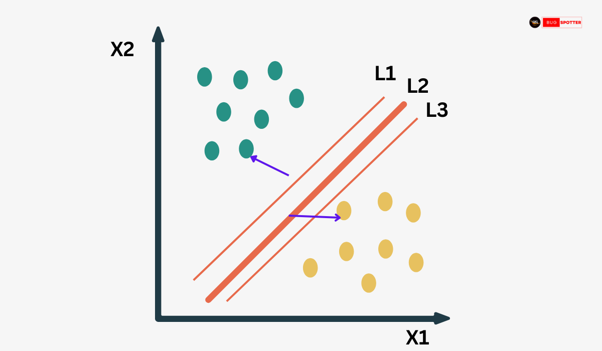
Two Classes of Data Points

Green Dots (Upper Left Region) → Represent one class.
Yellow Dots (Lower Right Region) → Represent another class.

Axes (X1, X2)

X1 (Horizontal Axis) and X2 (Vertical Axis) represent the two features of the dataset.
Each data point corresponds to a value of X1 and X2.

Three Lines (L1, L2, L3)

These lines represent possible hyperplanes (decision boundaries) that could separate the two classes.
Among them, L2 (middle line, bold red) is the optimal hyperplane found by SVM.
L1 and L3 are the margin boundaries that define the distance from the hyperplane to the closest data points, known as support vectors (indicated by purple arrows).

How SVM Works in This Scenario

Finding the Optimal Hyperplane (L2)

SVM aims to maximize the margin (the distance between the hyperplane and the nearest data points of each class).
The optimal hyperplane (L2) is placed right in the middle of the margin.

Role of Support Vectors

The closest data points from each class (indicated by arrows) are called support vectors.
These support vectors define the margin and influence the placement of the hyperplane.

Why L2 is the Best Hyperplane?

- L1 (above L2) and L3 (below L2) are not optimal because they are too close to one of the classes, reducing the margin.
A larger margin improves generalization, meaning the model performs better on unseen data.

Non-Linear SVM

A Non-Linear SVM (Support Vector Machine) is used when data cannot be separated by a straight line (or hyperplane in higher dimensions). Instead of trying to separate the data in its original space, Non-Linear SVM transforms the data into a higher-dimensional space where a linear separation becomes possible. This transformation is achieved using something called a Kernel Trick.

Why Do We Need Non-Linear SVM?

Consider a dataset where two classes (e.g., red and blue points) are mixed in such a way that no straight line can separate them. For example:

If the data is arranged in a circular pattern, a straight line will not work.
If the data follows a spiral shape, a simple hyperplane is useless.

In such cases, Linear SVM fails because it only finds straight boundaries. That’s where Non-Linear SVM comes in—it maps the data into a higher-dimensional space where a straight-line separation becomes possible.

How Does Non-Linear SVM Work?

Step 1: Feature Transformation
Instead of working with the original features (e.g., x and y), Non-Linear SVM creates new features to reshape the data.
These new features help SVM find a better decision boundary in a transformed space.
Step 2: Kernel Trick
Manually transforming data into a higher dimension is computationally expensive. Instead, we use a Kernel Function, which mathematically performs this transformation without explicitly computing the new dimensions.

Key Hyperparameters in SVM

C (Regularization Parameter)
Controls the trade-off between maximizing the margin and minimizing classification errors.
High C → More accuracy but less generalization.
Low C → Less accuracy but better generalization.
Kernel
Determines how data is transformed into a higher-dimensional space.
Common choices: Linear, Polynomial, RBF, Sigmoid.
Gamma (γ) in RBF Kernel
Determines how far a single training example influences the classification boundary.
High γ → Closer data points have more influence.
Low γ → Distant data points also have influence.

Advantages & Disadvantages of SVM

✅ Works well in high-dimensional spaces.
✅ Effective in cases where the number of features is greater than the number of samples.
✅ Uses a mathematical approach that ensures robustness.
✅ Can handle non-linear classification using kernel tricks.

Disadvantages

❌ Computationally expensive for large datasets.
❌ Requires careful tuning of hyperparameters like C and gamma.
❌ Not very effective when there is a lot of noise in the data.

Limitations of SVM

Slow for large datasets — computational cost is high.
Sensitive to noise — if there’s overlapping data, it can struggle.
Choosing the right kernel — picking the correct kernel is crucial for non-linear problems.

Latest Posts

All Posts
Software Testing
Uncategorized

End of Content.

Support Vector Machine in Machine Learning (SVM)